How to Perform Exploratory Data Analysis on a Loan Delinquency Problem -Part1

Hello readers!! We are back with another problem on machine learning and this time we are going to consider a numerical problem. Here we will focus on performing Exploratory data analysis (EDA) and refine the data. Next we will encode the categorical data to convert the entire data into numerical, then try different tree based machine learning algorithms and investigate which one has a better accuracy.

The Source of the problem about Loan Delinquency:

This problem is originally picked up from Data Science Foundation. You can visit this website which will require your registration. Alternatively, we are explaining the problem here as well.

Business Objective of this problem:

In the pursuit to assess the probability of loan default with respect to a customer, and thus identify the potential defaulters, the personal and credit details attached to that person applying for the loan needs to be furnished to the bank by the applicant. For a new application for loan, all the mentioned information might not be available with the bank. Here, lies the challenge to build up an effective statistical model to use the information furnished by the new applicant while applying for the loan, and to classify the applicant as a potential defaulter or non-defaulter. The objective here is to come up with an optimum model so that the number of correct classifications of potential defaulters and non-defaulters is maximized, for effective increase in profitability, or reduction of non-paying assets for the bank.

Data associated with this problem:

We are provided with Train_Data. The training data has around 11100+ records and 52 columns. The column Loan_Status = 0 signifies defaulters and a value 1 denotes non-defaulters. Various columns with its name and explanation is provided in the text file attached. Data_columns_explanation

Although in the original problem, we are provided with a Test data as well of around 4800 records, on which we have to apply our model and predict defaulters. We will stick to just the train data attached earlier. We will split in into a 75:25 train:test data and apply our model on the test data to find out its accuracy.

Knowledge Required:

Tiny bit of Python and understanding of various features of Pandas library,

Exploratory Data Analysis:

Its well known that as a practising Data Scientist, we do have to spend a majority of our time on Data Exploration, and cleaning. This is required so that we ensure the data is clean of all the missing values, outliers, junk characters or other unwanted data else these do hamper the accuracy of our models. So, fasten your seatbelts and put on your 3D glasses as we being exploring our data.

The excel sheet data is a well-structured data. Assuming you have downloaded and scanned the Loan Default data, some of the observations noticeable are as follows:

• Columns namely ID and Member_ID are unique customer ids. These two columns do not add any value/information to our data for a customer’s chances of defaulting. So, we will remove these two columns.
• The next column to be noticed is named TERM which has two values. They are 60 months and 30 months. We will convert the data such that only numerical value remains.
• Observing the Loan_Status columns tells us that only 351 customers defaulted out of around 11000+ customers. Clearly this is an unbalanced data. That is just 3.1 % of the customers have defaulted.
• The column EMP_TITLE holds various values like TEACHER, Teacher, teacher causing unnecessary unique values. We need to clean and organise these.
• The columns PYMNT_PLAN, POLICY_CODE and APPLICATION_TYPE is filled with just a single value. For example, APPLICATION_TYPE has INDIVIDUAL. This column does not add any information to our data because every customer is an INDIVIDUAL type. Hence, we will delete these columns.
• The columns ZIP_CODE needs to be cleaned and converted to just the numeric value. For example, 123xx will be converted to 123.
• There are several columns indicating dates like ISSUE_D, EARLIEST_CR_LINE, LAST_PYMNT_D, NEXT_PYMNT_D, LAST_CREDIT_PULL_D. What should we do about it? Can you think of something?
• We need to perform missing value analysis. Since in our case there are very negligible missing values, we will remove those records from the dataframe after identifying them.

We will be using pandas library extensively. First of all, we need to create a dataframe out of our excel file.

Next is the removal of columns named ID, Member_ID, PYMNT_PLAN, POLICY_CODE and APPLICATION_TYPE

Lets clean the columns TERM and ZIP_CODE as we explained earlier.

Missing values comprise of None, NaN (Not a Number). For columns which has date values, a 0 as date can also be considered as a missing value. Lets identify missing values in the whole dataframe. The screenshot shows which are those columns.

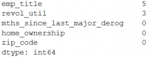
From the output we could see that there are just 5 missing values in the columns EMP_LENGTH and 3 in column REVOL_UTIL. Hence, we will proceed to remove these records with the following command.

In order to check availability of value 0 in a date valued column, we run the below command on the column. This will give us the count of zeros present. The result shows a total of 725 rows in the NEXT_PYMNT_D has a date value of 0. Similarly, we can change the column name in this command and find out the count for the remaining date columns.

Let us now explore the column ISSUE_D and see if we can refine it. The following command will give us the unique values present.

The result tells us that all the rows has date as 15^th. So, the only meaningful information we can pull out is the month value from this column which is from January to September. We will use string replace.

The unique values when checked shows – [‘Jul’, ‘Aug’, ‘Sep’, ‘Jan’, ‘Apr’, ‘Jun’, ‘Feb’, ‘Mar’, ‘May’]. Now the columns can be considered as a nominal data column. We can later apply one hot encoding to convert these into numerical values for model building.

We will be deleting the remaining 4 date columns since we assume that these are not adding any value to information in our date. But we can very well try and experiment for example separating out the year or quarter values. Do we have a better option? Hoping to see some discussion on this with interesting point of views from the readers.

Now let us explore the refined data frame for some insights. Our focus is only to investigate the records where loan_status=0. There are in total 351 such records. First thing is to slice the dataframe for the defaulting customers and then creating a new dataframe named df_defaulters separating them out

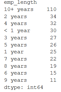
We will now do some grouping to see any patterns in the defaulters. First is to groupby on EMP_LENGTH column. The result shows that employees with >10 years of experience comprise of around 30% defaulters. The code and snapshot of its result is shown.

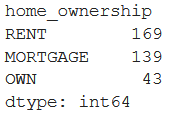
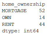
Now let us find out what kind of home do the defaulters own (column name HOME_OWNER)  and see if we see any pattern. The snapshot below clearly shows that the employees who live on RENT or on MORTGAGE contribute to 88% of the defaulters.

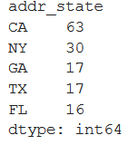
Similarly, we can gain some insight if we group by the column PURPOSE or DELINQ_2YRS or ADDR_STATE. Writing the code and the screenshot below.  From the first screenshot we can see that States CA and NY has around 26% defaulters.

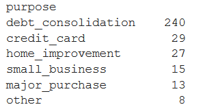
By checking the PURPOSE column we find that debt_consolidated is the most prominent purpose of the defaulters and amounts to 67% approx.

When we check the unique values in the column EMP_TITLE we can notice a lot of values like Manager, manager, account executive, account exec, Account Executive etc. Since all of these are considered unique values, we need to convert all the values to its lower case and then carefully clean these values so that the column data is refined and the count of unique values is accurate.  There are several kinds of managers like Account Manager, Sales Manager, Manager, A/R Manager etc. We will bring all of them to just one classification which is ‘manager’. Similarly for some other values, you can work on them as you find fit.  We have worked on cleaning some of the values and showed a part of it.

We can go deeper into grouping the defaulter’s data based on multiple columns and try to identify other patterns.Since we already identified that the EMP_LENGTH of +10 years has the most defaulters, lets go deep from there and combine HOME_OWNERSHIP to see what it reveals.

The snapshot above reveals that employees with more than 10+ years of experience who own their home defaults the least. Merely 14 out of the total 351 defaulters. anyways, only 43 out of 351 home owners defaulted.

Scatter Plot

Lets try some scatter to create some visuals for analysis. A scatterplot between ANNUAL_INC and FUNDED_AMNT can be found with the below command.

The output looks like this.

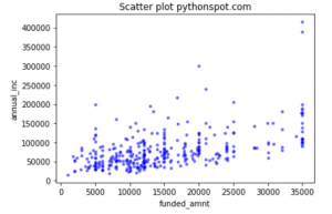
Lets check the correlation between these two columns with the below command. The result shows a positive correlation of .514.

A scatter plot on the whole dataframe for the same columns ANNUAL_INC and FUNDED_AMT looks something like below. The correlation between the two columns for the complete dataframe df_train drops to .409

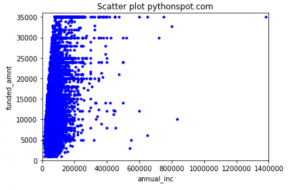
If you have noticed, both the plots provide a hint on the outliers. Do we need to do something about it? Hoping to see some discussion with interesting point of views from the readers.

Summary:

In this post we have tried to explain with examples and code the various ways of exploring data. Missing values, scatter plots, groupby, working on dates, using regular expressions etc. With this, we have paved the path towards encoding the categorical data and then proceed to modeling.  Please feel free to provide suggestion of improvements or on doing data exploration in a better way. Would be happy to learn and improve the post.

What next:

In the next post, as already said, we will explain various encoding like one hot, label, binary, etc and implement these in our data along with providing codes. We will also explore the option of normalizing the numeric columns and how might it impact the modeling. Thereafter, we are aiming to explain and work on the tree based models like Decision Tree and XGboost classifiers on the split of our train data available. Till then, Enjoy with the data!