Hope the previous article on exploration of the Loan Default data was informative. As stated, it is time to talk about encoding of a few categorical columns in our data.

In this article we will try to understand about encoding and importance of applying Machine Learning Tree Based Algorithms (Decision tree, Random Forest and XGBoost methods ) on a Loan Delinquency Problem and generate higher accuracy.

What is Encoding?

Encoding is a method with which we transform nominal or ordinal data columns into its numerical values. For example, assume a column color which has three values namely Blue, Red and Green.  It’s a nominal data. After applying some encoding rule, we convert the values to 1, 2 and 3 respectively.

Did you observe any issue with this conversion? There are various methods with which we can perform encoding on a categorical data like Label, One-hot, Binary, Hashing, Frequency etc.

Why do we need Encoding?

Machine learning models reads only numerical data and hence we need all the categorical/ non-numeric data to be changed into numbers before we proceed to apply any machine learning algorithm.

We will focus on 2 types of encoding namely Label and one-hot encoding.

Label Encoding

This type of encoding is used to convert an ordinal data column into its numeric values. For example, consider a field named Income Group having values Low Income Group (LIG) and High-Income Group (HIG). This is an ordinal data and we can use Label Encoding here. The Input and Output sample is shown below.

Input	Output
LIG	0
HIG	1

One-Hot Encoding

This type of encoding is used to convert a nominal data column into its numeric values. For example, consider a field named Colour having values Black and Blue. This is a nominal data and we can use one-hot encoding here with which we can get two binary features because of two values. The Input and Output sample is shown below.

Input	Red	Blue
Red	1	0
Blue	0	1

Now let us go back to our data frame, analyse which columns are categorical and what should be the course of action for those columns. The columns ‘Title’ and ‘Purpose’ are having same values. So, we will remove ‘Title’ column. Even though we removed the characters ‘xx’ from the zip code column values as shown in our last post, it is still a nominal data and not a numeric/ordinal data as it may look like.

These zip codes are grouped to its address state. Hence, we will remove the zip code column altogether and use one hot encoding on the addr_state column. The sub_grade column keeps finer details of the values in the field named ‘grade’ hence we can get rid of grade column. The most messed column is the emp_title column for which we did perform some cleaning previously.

Now when we check the total number of unique vales, it still comes around 4100 values. This means we need to go ahead and do another round of refining on this column which will be a tedious and time-consuming task. Hence, we will remove this column from the data frame. You can very well go ahead and clean this column as much as you want after which you will need to apply encoding on it. ( Suggestions on this in the comment section is most welcome). Another column named ‘earliest_cr_line’ contains date on which the customer took his/her first loan. We can retain only the year out of the values and apply one-hot encoding considering the values as nominal data.

This will need that we ensure proper data format in the excel itself. Our data frame column value looks like the below snapshot. Therefore, we will get this removed because the first and the 5^th value does not contain year.

You can use the below command to find out the number of unique values in the column emp_title.

After all these cleaning we now have 8 remaining categorical data columns on which we should proceed with the encoding. In our understanding we can consider all of these as nominal except emp_length which provide years of employment. Let us use Label encoding for this column.

When we see the output, the numeric values assigned are as follows:

10+ years	1
<1 year	10
1 years	0
2 years	2
3 years	3
4 years	4
5 years	5
6 years	6
7 years	7
8 years	8
9 years	9

Does this look correct? No, this does not look correct because of the numerical value assigned for 10+ years is 1 whereas for <1 year is 10. This needs to be corrected. Hence, we will simply keep only the numeric value from the column values and remove all the characters and special characters. This will automatically convert the column into a numeric valued column respective of the year of employment.

This column emp_length is an integer data type. We will use the following basic commands to clean all characters except the digits. Would like the readers to suggest a better command. Do check the data type of the column after editing.

The remaining 7 columns are nominal, and we will be applying one-hot encoding on those columns.

Feature importance –

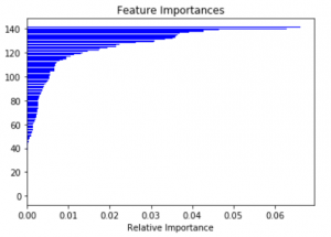
Let us now work on the feature importance. This tells us how important a feature is in impacting the outcome which in our case is loan_status. We will use decision tree classifier and generate a plot of feature importance with the code provided as follows.

From the graph its visible that only approx. top 40 to 50 features impact the loan_status with more than 1% importance. Rest all the featured have negligible impact and hence our next action will be to filter out low importance columns from the data frame. This will reduce the size and volume of our data frame and the model computation.

Let us see those 40-50 features clearly with the below commands.

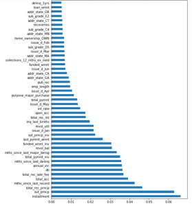
We will proceed with keeping just these columns in the data frame.

Data split –

Its time to split the data frame into 80:20 train and test data set.

We are going to apply three algorithms. Decision tree, Random Forest and XGBoost methods and see which one proves more accurate.

1. Decision tree model –

   Decision tree

   Python

   from sklearn import tree model.fit(X_train,y_train) df_test_output= model.predict(X_test) import numpy as np np.unique(df_test_output, return_counts=True) np.unique(y_test, return_counts=True) from sklearn.metrics import accuracy_score accuracy_score(y_test, df_test_output)

   1 2 3 4 5 6 7 8 9 10

   from sklearn import tree model.fit(X_train,y_train) df_test_output= model.predict(X_test)   import numpy as np np.unique(df_test_output, return_counts=True) np.unique(y_test, return_counts=True)   from sklearn.metrics import accuracy_score accuracy_score(y_test, df_test_output)

2. Random Forest model –

   Random Forest

   Python

   from sklearn.ensemble import RandomForestClassifier model= RandomForestClassifier(n_estimators=100) from sklearn import tree model.fit(X_train,y_train) df_test_output= model.predict(X_test) import numpy as np np.unique(y_test, return_counts=True) np.unique(df_test_output, return_counts=True) from sklearn.metrics import accuracy_score accuracy_score(y_test, df_test_output)

   1 2 3 4 5 6 7 8 9 10 11 12

   from sklearn.ensemble import RandomForestClassifier model= RandomForestClassifier(n_estimators=100)   from sklearn import tree model.fit(X_train,y_train) df_test_output= model.predict(X_test) import numpy as np np.unique(y_test, return_counts=True) np.unique(df_test_output, return_counts=True)   from sklearn.metrics import accuracy_score accuracy_score(y_test, df_test_output)

3. XGBoost Classifier model –

   While working on this model, we will have to ensure that no columns are of string type in the data set. We edited two columns which were of the data type O. Would request you to go ahead and solve it when you face the issue.

   XGBoost

   Python

   !pip install xgboost import xgboost from numpy import loadtxt from xgboost import XGBClassifier # fit model no training data model = XGBClassifier() from sklearn import tree model.fit(X_train,y_train) df_test_output= model.predict(X_test) import pandas as pd import numpy as np np.unique(y_test, return_counts=True) np.unique(df_test_output, return_counts=True) from sklearn.metrics import accuracy_score accuracy_score(y_test, df_test_output)

   1 2 3 4 5 6 7 8 9 10 11 12 13 14 15 16 17

   !pip install xgboost import xgboost from numpy import loadtxt from xgboost import XGBClassifier # fit model no training data model = XGBClassifier()   from sklearn import tree model.fit(X_train,y_train) df_test_output= model.predict(X_test) import pandas as pd import numpy as np np.unique(y_test, return_counts=True) np.unique(df_test_output, return_counts=True)   from sklearn.metrics import accuracy_score accuracy_score(y_test, df_test_output)

   When you compare the accuracy of these three models, we have the below numbers.

   Model Name	Accuracy %
   Decision Tree	94.81
   Random Forest	97.23
   XGBoost	97.36

   Evidently, XGBoost generates the best accuracy. This model is the most popular model for winning the data science contests for various reasons. One of which is that it takes less time to compute in comparison with Random Forest. Also, a single decision tree implementation will conceptually have less accuracy over Random Forest because it gets rid of over fitting problem as it takes an average of all the decision tree predictions made behind the scene, thereby cancelling the bias.

   Conclusion:

   We have given a microscopic view of the various activities and tasks which needs to be done to make a data set eligible for applying algorithms. Also, on how to apply models and generate higher accuracy. We have kept the content such that the reader gets a very novice perspective of how to play with a data set, facing issues while working on something and then resolving it eventually enhancing the learning experience.

   Now, do you think our task is over? Or did you observe some pitfalls or points of improvement? Did you observe that our dataset was by large a skewed data set because the Training data set had just around 3% loan defaulters? Having said that, how can we enhance our model and refine the way in which we performed model fitting? Do you have any suggestion?

   Please do let us know in the comment section about your views, questions, doubts or any point you think is better than the one provided. Till then!