Sentiment Analysis of Tweets – Predicting Sentiments using Machine Learning Algorithms
Sentiment Analysis of Tweets:
This post is in continuation of the previous article where we created a twitter app and established a connection between R and the Twitter API via the app. In this article, we will Predict Sentiments by doing Sentiment Analysis of Tweets. Let us begin.
Since Wimbledon 2019 has ended some time ago, we will perform our sentiment analysis on the latest happening of Assam Floods by fetching tweets with #AssamFloods
|
1 |
Flood_tweets = search_tweets("#AssamFloods", n=3000, lang='en', include_rts=FALSE) |
When we check for the length of how many columns does the records fetched from the above command has, we find it 88.
![]()
Let us check what the first few columns are.
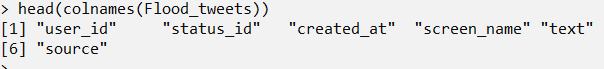
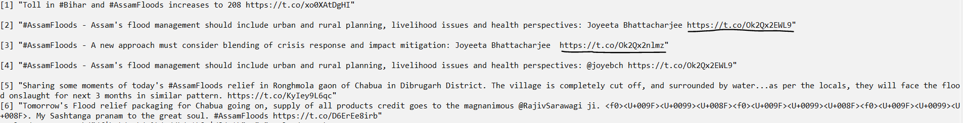
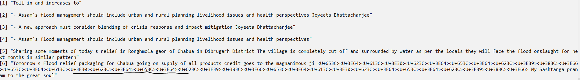
This tells us that the fifth column named ‘text’ is the one which is of our need. We will be exploring only this field hereafter. Let us look at how the tweets look like.

The text in the tweet looks like this.
“Natural calamities wreak havoc but humanity has the power to join hands and help others who are in need. Each one of us can do something to help the people in flood-hit Assam. Read on to find out:\nhttps://t.co/QiNssWgswx\n#CauseAChatter #AssamFloods https://t.co/5K0Jx7qyEQ”
This contains hashtags, weblinks. There can be other junk characters, tabs, and spaces, Islands, etc which can be present. All these need to be removed from our tweets for our lexicon-based sentiment analysis. We will clean our tweets and then proceed with the sentiment analysis.
Cleaning of Tweets
As already explained, the collected tweets will need cleaning of its hashtags, extra spaces, and tabs, alphanumerics, HTTP links in tweets, etc because they won’t amount to any sentiment hence the exclusion. First, let’s create a new object and populate it with just the tweets text from the Flood_tweets.
|
1 |
Flood_text= Flood_tweets$text |
We will be using the gsub function to perform data cleaning on this character variable Flood_text.
Although we have used the parameter include_rts=FALSE to exclude any retweets in fetching our tweets, we will remove retweet entities from the stored tweets (text).
|
1 |
Flood_text = gsub("(RT|via)((?:\\b\\W*@\\w+)+)", " ", Flood_text) |
# Remove HTML links. Not required for sentiment analysis. Underlined in the above image.
|
1 |
Flood_text = gsub("(f|ht)(tp)(s?)(://)(.*)[.|/](.*)", " ", Flood_text) |
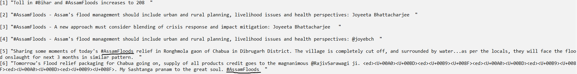
# Then remove all “#Hashtag”. Underlined in the above image.
|
1 |
Flood_text = gsub("#\\w+", " ", Flood_text) |
|
1 2 3 4 5 6 7 8 9 10 11 12 |
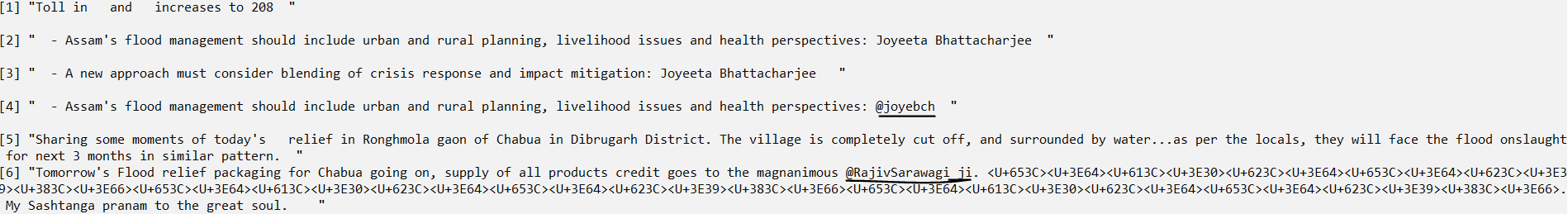
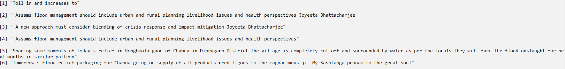
# Then remove all "@people". Underlined in the above image. Flood_text = gsub("@\\w+", " ", Flood_text) # Then remove all the punctuation. Underlined in the above image Flood_text = gsub("[[:punct:]]", " ", Flood_text) # Then remove numbers, we need only text for analytics Flood_text = gsub("[[:digit:]]", " ", Flood_text) # Finally, we remove unnecessary spaces (white spaces, tabs etc) Flood_text = gsub("[ \t]{2,}", " ", Flood_text) Flood_text = gsub("^\\s+|\\s+$", "", Flood_text) |
The above, underlined junk character is UTF-8 type. We remove it by using the below command.
|
1 |
Flood_text = iconv(Flood_text, "UTF-8", "ASCII", sub="") |
Let us clean the tweets if we somehow got everything in the tweet removed and all that remains is a NA (Not available).
|
1 2 3 |
Flood_text = Flood_text[!is.na(Flood_text)] names(Flood_text) = NULL Flood_text = unique(Flood_text) |
Our tweets’ text data is cleaned now. The next job is to identify the sentiment of tweets which can be either Positive, Negative, or Neutral. For this, we will use an inbuilt function classify_polarity available in the ‘sentiment’ package.
Alternatively, what we could do is manually identify sentiments of the tweets and then use that to train the machine learning model so that it would then predict sentiments of the test tweets. Here we will resort to the prior method.
|
1 2 3 |
install.packages(“sentiment”) library(sentiment) Flood_text_pol = classify_polarity(Flood_text, algorithm="bayes") |
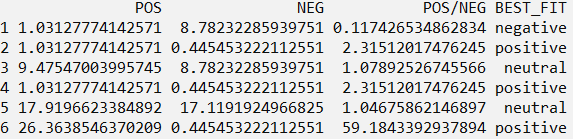
What this function does is from a lexicon of positive and negative words, it compares every word from a tweet text, gives positive and negative scores, and identifies the BEST_FIT as seen in the above screenshot. With this, we have got the sentiment of all the tweets we could collect for #AssamFloods.
Now, the main intention is to work on 2 different Machine Learning algorithms to predict sentiments of tweets and then check which one was more accurate. For this, we will split our tweet data set and use the first 1900 rows for training the model and the remaining 819 rows as test data to predict their sentiments.
Before applying a machine learning algorithm on any text data, we need to apply the Term Frequency – Inverse Document Frequency concept. For this, we will reduce irrelevant text from the corpus of tweets collected and generate a Document Term Matrix.
Document Term Matrix is a matrix that described the frequency of terms that occur in a set of documents. Its rows would correspond to the documents in the collection and columns would correspond to terms. In our case documents would mean tweets and hence 2310 documents.
|
1 2 3 4 5 6 |
Flood_text_Corpus<- Corpus(VectorSource(Flood_text)) Flood_text_Corpus<- tm_map(Flood_text_Corpus, removePunctuation) Flood_text_Corpus<- tm_map(Flood_text_Corpus, content_transformer(tolower)) Flood_text_Corpus<- tm_map(Flood_text_Corpus, removeWords, stopwords("english")) Flood_text_Corpus<- tm_map(Flood_text_Corpus, stripWhitespace) Flood_text_Dtm<- DocumentTermMatrix(Flood_text_Corpus) |
Let us now understand about Term Frequency and Inverse Document Frequency. It is like a measure to evaluate the importance of any word/term in a document in a collection of documents.
Term Frequency: This means what is the frequency of a term in a document.
Document Frequency: This tells how many different documents in which the term occurs.
Inverse Document Frequency: This is given by the total number of documents in the corpus divided by the document frequency.
We have 2310 documents. Let us say in the first document, the word ‘loss’ is used twice. That document consists of 15 words. So, its Term Frequency is 2/15=0.133. If this word occurs in say 1000 documents overall, then the Document Frequency is 1000. Its Inverse Document Frequency will be given by log10(2310/1000) = 0.36. The TF-IDF will be 0.133* 0.36 = 0.048
We are doing this calculation to offset any regular term like for example ‘the’ which would be most present in every document and hence would come as a high importance word while it does add nothing to help identify the document’s sentiment.
We will create three different functions for Term Frequency, Inverse Document Frequency, and Term Frequency – Inverse Document Frequency as shown below.
|
1 2 3 4 5 6 7 8 9 |
term_frequency<- function(term){term/sum(term)} inverse_document_frequency<- function(document){ corpus_size<- length(document) document_count<- length(which(document>0)) log10(corpus_size/document_count) } term_freq_inv_doc_freq<- function(term_f,inv_doc_f){ term_f*inv_doc_f} |
Now let us apply the TF-IDF on our tweets.
|
1 2 3 4 5 6 7 8 9 10 |
Flood_text_Dtm_tf<- apply(Flood_text_Dtm, 1, term_frequency) Flood_text_Dtm_idf<- apply(Flood_text_Dtm, 2, inverse_document_frequency) Flood_text_Dtm_tfidf<- apply(Flood_text_Dtm_tf,2, term_freq_inv_doc_freq, inv_doc_f = Flood_text_Dtm_idf) Flood_text_Dtm_tfidf<- t(Flood_text_Dtm_tfidf) incomplete.cases<- which(!complete.cases(Flood_text_Dtm_tfidf)) Flood_text_Dtm_tfidf[incomplete.cases,]<- rep(0.0, ncol(Flood_text_Dtm_tfidf)) dim(Flood_text_Dtm_tfidf) sum(which(!complete.cases(Flood_text_Dtm_tfidf))) Flood_text_polarity= cbind(Flood_text, Flood_text_pol[,4]) Flood_text_Dtm_tfidf.df<- cbind(Flood_text_polarity, data.frame(Flood_text_Dtm_tfidf)) |
We apply supervised machine learning algorithms as we have training data available with us for the algorithm to learn from. The first algorithm is K-Nearest Neighbours (KNN) classification because we want to classify tweets into positive, negative, and neutral sentiments.
What is KNN Algorithm?
The K Nearest Neighbours is an algorithm that would require to pass a value of K (number of neighbors). With that, every new test point is measured as per its distance with the pre-determined neighbors, the nearest neighbor is identified, and a classification is made/predicted.
The measurement of distance can be Euclidean or Manhattan or Minkowski etc. We install a package named class to predict the sentiments of the test tweets using KNN. We have split our data in the ration of 70:30 and hence training data is of 1600 tweet texts and test data is of the remaining 710 tweet texts.
|
1 2 3 4 5 |
install.packages(“class”) library(class) Flood_text_Train<- (Flood_text_Dtm_tfidf[1:1600,]) Flood_text_Test<- (Flood_text_Dtm_tfidf[1601:2310,]) |
Let us work with three different K values (10, 5, and 3) and analyze which one is more accurate.
|
1 2 3 |
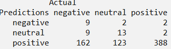
Flood_text_Pred<- knn(Flood_text_Train, Flood_text_Test, Flood_text_pol[1:1600,4], k=10) conf.matrix<- table("Predictions"= Flood_text_Pred, "Actual"= Flood_text_pol[1601:2310,4]) |
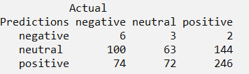
Out of the total 710 test tweets, we see that 246+63+6=315 predictions were accurate.
|
1 2 3 |
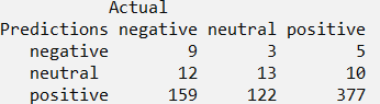
Flood_text_Pred<- knn(Flood_text_Train, Flood_text_Test, Flood_text_pol[1:1600,4], k=5) conf.matrix<- table("Predictions"= Flood_text_Pred, "Actual"= Flood_text_pol[1601:2310,4]) |
Out of the total 710 test tweets, we see that 388+13+9=410 predictions were accurate.
|
1 2 3 |
Flood_text_Pred<- knn(Flood_text_Train, Flood_text_Test, Flood_text_pol[1:1600,4], k=3) conf.matrix<- table("Predictions"= Flood_text_Pred, "Actual"= Flood_text_pol[1601:2310,4]) |
Out of the total 710 test tweets, we see that 377+13+9=399 predictions were accurate.
Based on these results we can decide which K value will be the most suitable for us in terms of arriving at more accurate predictions. If we have a greater number of tweets to train and test, the results would improve.
Now let us move to another algorithm which is called Random Forest.
What is a Random Forest?
Random Forest is another supervised machine learning algorithm that can be used for classification as well as regression. This algorithm creates a forest with n number of trees which we can pass as a parameter. Random Forest is a step further to the Decision Tree algorithm.
A decision tree is a very popular supervised machine learning algorithm that works well with classification as well as regression.
It starts from a root node and ends at a leaf node (decision) by carefully splitting into branches based on conditions (decision node) and moving forward until a final decision is reached. The splits happen based on the decision node which provides the largest information gain or decreases entropy.
We would suggest that the reader tries sentiment classification using Decision Tree with 1 or more trees and analyze the accuracy of results. Let us now see how a Random Forest works.
|
1 2 3 4 5 6 7 8 9 |
install.packages(“randomForest”) library(randomForest) Flood_RF=randomForest(x=Flood_text_Dtm_tfidf.df[1:1600,3:4871], y=Flood_text_Dtm_tfidf.df[1:1600,2] , ntree=10, keep.forest=TRUE) Flood_text_Pred= predict(Flood_RF, Flood_text_Dtm_tfidf.df[1601:2310, 3:4871]) conf.matrix<- table("Predictions"= Flood_text_Pred, "Actual"= Flood_text_Dtm_tfidf.df[1601:2310,2]) conf.matrix |
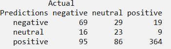
Out of the total 710 test tweets, we see that 364+23+69=456 predictions were accurate.
|
1 2 3 4 5 6 |
Flood_RF=randomForest(x=Flood_text_Dtm_tfidf.df[1:1600,3:4871], y=Flood_text_Dtm_tfidf.df[1:1600,2] , ntree=5, keep.forest=TRUE) Flood_text_Pred= predict(Flood_RF, Flood_text_Dtm_tfidf.df[1601:2310, 3:4871]) conf.matrix<- table("Predictions"= Flood_text_Pred, "Actual"= Flood_text_Dtm_tfidf.df[1601:2310,2]) conf.matrix |
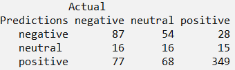
Out of the total 710 test tweets, we see that 349+16+87=452 predictions were accurate.
Clearly, the Random Forest algorithm gives better sentiment prediction than the KNN approach.
We can also implement Deep Learning techniques to get the sentiments for example in the case of identifying the sentiment of IMDB review comments. In order to prepare our text data, we need to apply the word embedding concept of NLP.
Thereafter we can apply a one-dimensional convolutional neural network model or a simple multi-layer Perceptron Model for sentiment analysis. The explanation of which is beyond the scope of this article.
Do tell us if you face any difficulty in understanding anything, have any suggestions for improvements, any doubts, etc.


Hello! Thanks for a great guide. Iam trying to run the script: Flood_text_pol = classify_polarity(Flood_text, algorithm=”bayes”). It keeps returung at error:Error in classify_polarity(Flood_text, algorithm = “bayes”, prior = 1) :
could not find function “classify_polarity”. When I install package sentiment, I get thiserror: Warning in install.packages :
package ‘sentiment’ is not available (for R version 3.6.2)
Can you please help?
Sure, Brian. Yes. This package was archived long back in December 2012. To install sentiment package will also require packages tm and Rstem(this package is also archived). You can follow the below steps to install it.
1) require(devtools)
2) packageurl <- "http://www.omegahat.net/Rstem/Rstem_0.4-1.tar.gz"
3) install.packages(packageurl, repos=NULL)
4) install.packages("tm")
5) packageurl <- "https://cran.r-project.org/src/contrib/Archive/sentiment/sentiment_0.1.tar.gz"
install.packages(packageurl, repos=NULL)
Please let me know if further help is needed.
Dear Rounak, can you tell me how label the tweets for training purpose?
Hi Naganna, sure. I think you are asking how can we label the tweets as positive, negative and neutral. I have pointed that out either we can manually label them which will be very time-consuming. Alternatively, we have used a function from ‘sentiment’ package which labels the tweets into positive, negative and neutral. This is not very accurate but for generating a basic understanding of text analytics we have worked on that in the blog.
Please let us know if you need further clarification.
Nice guide. But for some reason, my script wont download more than 5-12 columns. I’ve tried everything from changing the hashtag, changing all the parameters, regenerating my API-keys but nothing works.
Do you have any ideas what’s going on? Is my developer account setup wrong? I did everything as you’re supposed to do, but I feel like I’m being severely limited.
Hi DonK. Thanks for sharing your issue. Can you provide the command and share more info about the result? There are supposed to be 88 columns of data for each tweet when we use search_tweets command. Should not be any problem due to dev account setup.